Chapter 6 Spatial Analysis in R
“Why are latitude and longitude so smart? Because they have so many degrees!”
In this assignment, I learned to use R for spatial analyses.
Data is from the LAGOS dataset. Assignment by Dr. Matthew Ross and Dr. Nathan Mueller of Colorado State University.
6.1 Loading in data
6.1.1 First download and then specifically grab the locus (or site lat longs)
# #Lagos download script
#LAGOSNE::lagosne_get(dest_folder = LAGOSNE:::lagos_path(), overwrite = TRUE)


#Load in lagos
lagos <- lagosne_load()
## Warning in (function (version = NULL, fpath = NA) : LAGOSNE version unspecified,
## loading version: 1.087.3#Grab the lake centroid info
lake_centers <- lagos$locus
# Make an sf object
spatial_lakes <- st_as_sf(lake_centers,coords=c('nhd_long','nhd_lat'),
crs=4326)
#Grab the water quality data
nutr <- lagos$epi_nutr
#Look at column names
#names(nutr)6.1.2 Convert to spatial data
#Look at the column names
#names(lake_centers)

#Look at the structure
#str(lake_centers)

#View the full dataset
#View(lake_centers %>% slice(1:100))

spatial_lakes <- st_as_sf(x = lake_centers, coords = c("nhd_long","nhd_lat"), crs = 4326) %>%
  st_transform(2163)

#mapview(spatial_lakes)

#Subset for plotting
subset_spatial <- spatial_lakes %>%
  slice(1:100)

subset_baser <- spatial_lakes[1:100,]

#Dynamic mapviewer
#mapview(subset_spatial)
6.1.3 Subset to only Minnesota
states <- us_states()

#Plot all the states to check if they loaded
#mapview(states)

minnesota <- states %>%
  filter(name == 'Minnesota') %>%
  st_transform(2163)
#mapview(minnesota)

#Subset lakes based on spatial position
minnesota_lakes <- spatial_lakes[minnesota,]

#Plotting the first 1000 lakes
minnesota_lakes %>%
  arrange(-lake_area_ha) %>%
    slice(1:1000)
## Simple feature collection with 1000 features and 16 fields
## Geometry type: POINT
## Dimension: XY
## Bounding box: xmin: 254441 ymin: -154522.4 xmax: 755222.3 ymax: 464949.4
## Projected CRS: NAD27 / US National Atlas Equal Area
## First 10 features:
## lagoslakeid nhdid gnis_name lake_area_ha lake_perim_meters
## 1 15162 123319728 Lake of the Woods 123779.817 401005.02
## 2 34986 105567868 Lower Red Lake 66650.332 115825.47
## 3 2498 120019294 Mille Lacs Lake 51867.225 151701.94
## 4 39213 105567402 Upper Red Lake 48288.325 99828.05
## 5 996 120018981 Leech Lake 41824.352 344259.98
## 6 583 120019513 Lake Winnibigoshish 22566.124 86722.10
## 7 73 120019354 Rainy Lake 18522.551 660313.32
## 8 2554 105954753 Vermilion Lake 15736.590 509617.01
## 9 2161 120019371 Kabetogama Lake 9037.249 288750.31
## 10 3119 166868528 Cass Lake 8375.173 85326.14
## nhd_fcode nhd_ftype iws_zoneid hu4_zoneid hu6_zoneid hu8_zoneid hu12_zoneid
## 1 39004 390 IWS_37547 HU4_26 HU6_36 HU8_468 HU12_13912
## 2 39004 390 IWS_34899 HU4_54 HU6_74 HU8_327 HU12_14600
## 3 39004 390 IWS_22933 HU4_25 HU6_73 HU8_344 HU12_10875
## 4 39004 390 IWS_33471 HU4_54 HU6_74 HU8_327 HU12_14204
## 5 39004 390 IWS_23572 HU4_25 HU6_35 HU8_332 HU12_14479
## 6 39004 390 IWS_22455 HU4_25 HU6_35 HU8_331 HU12_14543
## 7 39004 390 IWS_37542 HU4_26 HU6_36 HU8_473 HU12_13942
## 8 39004 390 IWS_36424 HU4_26 HU6_36 HU8_131 HU12_14405
## 9 39004 390 IWS_36301 HU4_26 HU6_36 HU8_130 HU12_14395
## 10 39004 390 IWS_21080 HU4_25 HU6_35 HU8_331 HU12_13957
## edu_zoneid county_zoneid state_zoneid elevation_m geometry
## 1 EDU_56 County_435 State_14 323.5090 POINT (366706.2 464949.4)
## 2 EDU_16 County_455 State_14 358.1656 POINT (371974.2 341706.5)
## 3 EDU_43 County_484 State_14 381.7920 POINT (489582.1 157109.5)
## 4 EDU_16 County_455 State_14 358.3096 POINT (389013.3 360819.5)
## 5 EDU_42 County_424 State_14 395.2420 POINT (422409.7 255724.9)
## 6 EDU_42 County_424 State_14 396.1560 POINT (437872.1 286675)
## 7 EDU_55 County_446 State_14 338.0670 POINT (515833.6 420274.2)
## 8 EDU_3 County_446 State_14 414.1680 POINT (566966.7 347059.1)
## 9 EDU_55 County_446 State_14 339.2530 POINT (519199.2 408290.2)
## 10 EDU_42 County_424 State_14 396.7710 POINT (410563.2 281005.2) #mapview(.,zcol = 'lake_area_ha')6.2 Part one
6.2.1 Show a map outline of Iowa and Illinois (similar to Minnesota map upstream)
Istates <- states %>%
  filter(name == 'Iowa'| name== 'Illinois') %>%
  st_transform(2163)
mapview(Istates, canvas = TRUE)
6.2.2 Subset LAGOS data to these sites, how many sites are in Illinois and Iowa combined? How does this compare to Minnesota?
Istates_lakes <- spatial_lakes[Istates,]

nrow(Istates_lakes)
## [1] 16466Istates_count <- length(Istates_lakes$lagoslakeid)
nrow(minnesota_lakes)## [1] 29038Minn_count <- length(minnesota_lakes$lagoslakeid)Iowa and Illinois have 16466 lakes combined, much less than the number of lakes that Minnesota alone has, 29038.
6.2.3 What is the distribution of lake size in Iowa vs. Minnesota?
- Here I want to see a histogram plot with lake size on x-axis and frequency on y axis (check out geom_histogram)
iowa <- states %>%
  filter(name == 'Iowa') %>%
  st_transform(2163)

iowa_lakes <- spatial_lakes[iowa,]

combined <- rbind(iowa_lakes, minnesota_lakes)

ggplot(combined, aes(x= lake_area_ha)) +
  ggthemes::theme_few() + theme(legend.position="bottom") +
  xlab("Lake Area (ha)") + ylab("Count") +
  scale_x_continuous(trans = "log10", labels = scales::comma) +
  geom_histogram(data = minnesota_lakes, color = "red", alpha = 0.2) +
  geom_histogram(data = iowa_lakes, color = "blue", alpha = 0.2) +
  scale_fill_manual(values=c("blue","red"), "State")
## `stat_bin()` using `bins = 30`. Pick better value with `binwidth`.
## `stat_bin()` using `bins = 30`. Pick better value with `binwidth`.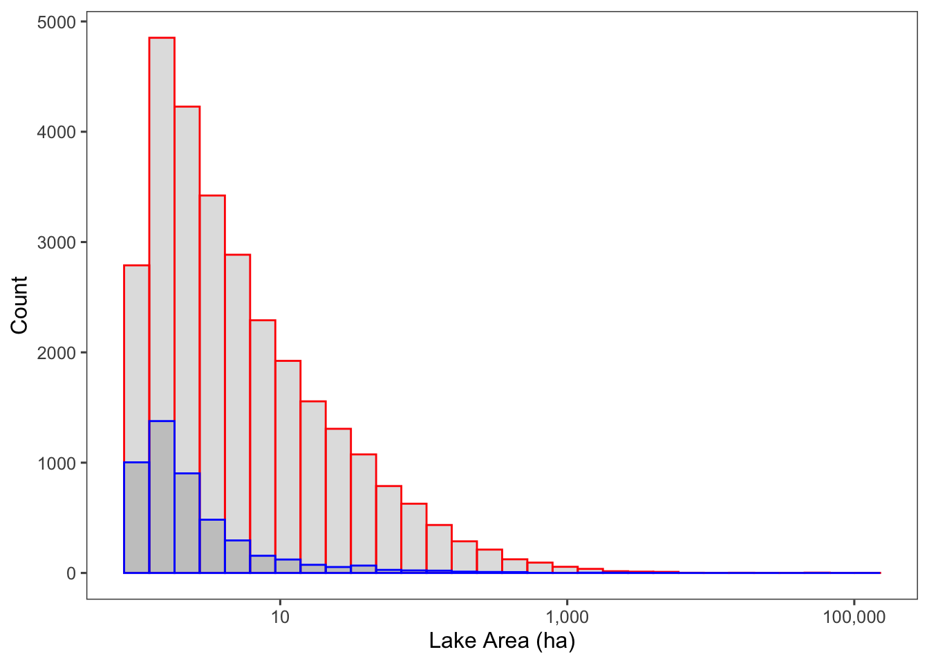
Figure 6.1: The number of lakes with a given area, in hectares, in Minnesota (red) and Iowa (blue).
6.2.4 Make an interactive plot of lakes in Iowa and Illinois and color them by lake area in hectares
Istates_map = Istates_lakes %>%
  arrange(-lake_area_ha) %>%
    slice(1:1000)

mapview(Istates_map, zcol = 'lake_area_ha',  canvas = TRUE)
6.2.5 What other data sources might we use to understand how reservoirs and natural lakes vary in size in these three states?
We might use the US Geological Survey (USGS) National Water Informational System (NWIS) and its National Water Dashboard as a data source, and look at gage height (indicating lake depth) as another parameter for lake size variation. The USGS National Hydrography Dataset (NHD) is another data source that would, similarly to Lagos, give us a surface area metric for lakes in the various states.
6.3 Part two
6.3.1 Subsets
6.3.1.1 Columns nutr to only keep key info that we want
clarity_only <- nutr %>%
  dplyr::select(lagoslakeid,sampledate,chla,doc,secchi) %>%
  mutate(sampledate = as.character(sampledate) %>% ymd(.))
6.3.1.2 Keep sites with at least 200 observations
#Look at the number of rows of dataset
#nrow(clarity_only)

chla_secchi <- clarity_only %>%
  filter(!is.na(chla),
         !is.na(secchi))

# How many observatiosn did we lose?
# nrow(clarity_only) - nrow(chla_secchi)


# Keep only the lakes with at least 200 observations of secchi and chla
chla_secchi_200 <- chla_secchi %>%
  group_by(lagoslakeid) %>%
  mutate(count = n()) %>%
filter(count > 200)6.3.2 Mean Chlorophyll A map
### Take the mean chl_a and secchi by lake

means_200 <- chla_secchi_200 %>%
  # Take summary by lake id
  group_by(lagoslakeid) %>%
  # take mean chl_a per lake id
  summarize(mean_chl = mean(chla,na.rm=T),
            mean_secchi=mean(secchi,na.rm=T)) %>%
  #Get rid of NAs
  filter(!is.na(mean_chl),
         !is.na(mean_secchi)) %>%
  # Take the log base 10 of the mean_chl
  mutate(log10_mean_chl = log10(mean_chl))

#Join datasets
mean_spatial <- inner_join(spatial_lakes,means_200,
                          by='lagoslakeid')

#Make a map
mapview(mean_spatial, zcol='log10_mean_chl', layer.name = "Mean Chlorophyll A Content")
6.3.3 What is the correlation between Secchi Disk Depth and Chlorophyll a for sites with at least 200 observations?
ggplot(means_200) +
  geom_point(aes(mean_secchi, mean_chl)) +
  ggthemes::theme_few() +
  xlab("Mean Secchi Disk Depth") + ylab("Mean Chlorophyll Content")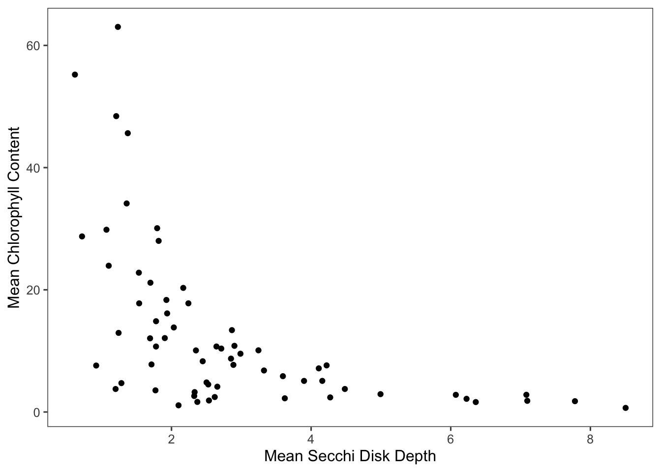
Figure 6.2: Chlorophyll content has a negative correlation with Secchi disk depth at sites with at least 200 observations.
6.3.3.1 Why might this be the case?
Secchi disks measure water clarity; the deeper the disk, the clearer the water (1). Chlorophyll content in lakes is generally a reliable marker of algae content, so that high chlorophyll values indicate high algal biomass and corresponding low water clarity (2). Additionally, chlorophyll may be used as a proxy for water quality, since high algal biomass is associated with high nutrient pollution in the process of eutrophication (2). High pollution may further decrease water clarity, so that the relationship between chlorophyll and Secchi disk depth may be expected.
“The Secchi Dip-in - What Is a Secchi Disk?” North American Lake Management Society (NALMS), https://www.nalms.org/secchidipin/monitoring-methods/the-secchi-disk/what-is-a-secchi-disk/.
Filazzola, A., Mahdiyan, O., Shuvo, A. et al. A database of chlorophyll and water chemistry in freshwater lakes. Sci Data 7, 310 (2020). https://doi-org.ezproxy2.library.colostate.edu/10.1038/s41597-020-00648-2
6.3.4 What states have the most data?
6.3.4.1 Make a lagos spatial dataset that has the total number of counts per site.
site_counts <- chla_secchi %>%
  group_by(lagoslakeid) %>%
  mutate(count = n())

lake_counts <- inner_join(site_counts, lake_centers, by= "lagoslakeid")%>%
  dplyr::select(lagoslakeid,nhd_long,nhd_lat, count, secchi, chla)

spatial_counts <- st_as_sf(lake_counts,coords=c("nhd_long","nhd_lat"),
                          crs=4326)
6.3.4.2 Join this point dataset to the us_boundaries data.
states <- us_states()

states_counts <- st_join(spatial_counts, states)
6.3.4.3 Group by state and sum all the observations in that state and arrange that data from most to least total observations per state.
sum_statecount <- states_counts %>%
  group_by(state_name) %>%
  summarize(sum = sum(count)) %>%
  arrange(desc(sum))

sumtable <- tibble(sum_statecount)

view(sumtable)

#ggplot(data = sumtable, aes(x=state_name, y=sum, fill=state_name)) +
#  geom_bar(stat = "identity", width = 0.3, position = "dodge") +
#  ggthemes::theme_few() +
#  xlab("State") + ylab(expression(paste("# of Observations")))
Minnesota has the most observations. Vermont, has the next most observations, but less than half of Minnesota’s observations. South Dakota has the least number of observations in the dataset.