Chapter 9 Evaluating Model Predictions

“Being a statistician means never having to say you are certain.”

In environmental sciences, it can be extremely valuable to not only try to parse out correlations and “peer inside the black box” to explain phenomena, but to also try to predict outcomes based on specific inputs and parameters. Equally important when we try to model predictions is to evaluate how well our model performs and predicts data. For this chapter, I looked at predictions from the CENTURY Model and evaluated how well the model fit with observed corn and wheat yield data from 1999-2013.

Data and assignment provided by Dr. Michael Lefsky of Colorado State University.

9.1 Merge model predictions and observed data

# Load datasets

#Century Model output through 2016
centgrain <- read.csv("Data_sci_bookdown/data/model-assess/century_harvest.csv")

centgrain13 <- centgrain[-c(16:18),] #Century model outputs through 2013

centwheat <- centgrain13 %>%
  filter(Crop == "wheat") #just the wheat outputs

centcorn <- centgrain13 %>%
  filter(Crop == "corn") #just the corn outputs

#load observed data
obsgrain <- read.csv("Data_sci_bookdown/data/model-assess/obs_corn_wheat_cgrain.csv") #observed data through 2013

obswheat <- obsgrain %>%
  filter(Crop == "wheat") #just the wheat outputs

obscorn <- obsgrain %>%
  filter(Crop == "corn") #just the corn outputs

#merge data from Century Model and observations
wheat <- merge(centwheat,obswheat, by=c('Year','Crop'), all.x = T) # merge predicted and observed wheat yields
corn <- merge(centcorn,obscorn, by=c('Year','Crop'), all.x = T) # merge predicted and observed wheat yields
allgrain <- merge(centgrain13, obsgrain, by=c('Year','Crop'), all.x = T) # merge all predicted and observed

9.2 Linear regression model and ANOVA of wheat predictions vs. observations

lm_wheat <- lm(cgrain_cent ~ cgrain_obs, data = wheat) # linear model of predicted vs. observed wheat yields
summary(lm_wheat) # intercept, slope (estimate column), P, R^2

## 
## Call:
## lm(formula = cgrain_cent ~ cgrain_obs, data = wheat)
## 
## Residuals:
##     Min      1Q  Median      3Q     Max 
## -59.857  -2.631   6.911  14.383  25.962 
## 
## Coefficients:
##             Estimate Std. Error t value Pr(>|t|)   
## (Intercept) 512.0318   127.8900   4.004  0.00709 **
## cgrain_obs   -0.4359     0.3544  -1.230  0.26473   
## ---
## Signif. codes:  0 '***' 0.001 '**' 0.01 '*' 0.05 '.' 0.1 ' ' 1
## 
## Residual standard error: 28.83 on 6 degrees of freedom
## Multiple R-squared:  0.2014, Adjusted R-squared:  0.06827 
## F-statistic: 1.513 on 1 and 6 DF,  p-value: 0.2647

summary(aov(lm_wheat)) # ANOVA

##             Df Sum Sq Mean Sq F value Pr(>F)
## cgrain_obs   1   1257  1257.3   1.513  0.265
## Residuals    6   4986   831.1

ggplot(data = wheat, aes(x=cgrain_cent,y=cgrain_obs)) + 
  geom_point(color="black") + geom_smooth(method="lm", se=FALSE, color="#78917E") +
  xlab("Predicted Yields (g C/m2/yr)") + ylab(expression(paste("Observed Yields (g C/m2/yr)"))) + 
  ggtitle("Predicted vs. Observed Wheat Yields") +
  theme_few(base_size = 16)

## `geom_smooth()` using formula 'y ~ x'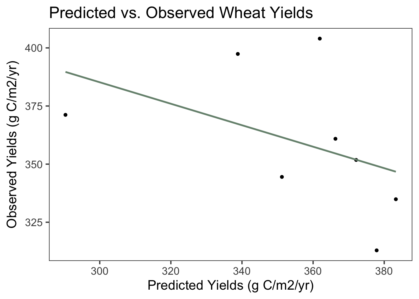

Figure 9.1: Scatterplot and linear regression line of predicted and observed wheat yields in grams of carbon (C) per m2 per year between 1999 and 2013. The equation of the line is -0.436x + 512, demonstrating that observed yields were lower than predicted yields on average. The multiple R2 value is 0. 201 and the adjusted R2 value is 0.0683, indicating a very weak linear relationship. The p-value is 0.265, considerably higher than what is generally considered to be significant.

9.3 Linear regression model and ANOVA of corn predictions vs. observations

lm_corn <- lm(cgrain_cent ~ cgrain_obs, data = corn) # linear model of predicted vs. observed corn yields
summary(lm_corn) # intercept, slope (estimate column), P, R^2

## 
## Call:
## lm(formula = cgrain_cent ~ cgrain_obs, data = corn)
## 
## Residuals:
##        1        2        3        4        5        6        7 
##  -7.7548  -0.1305 -16.2379 -18.3472  14.2575  14.2393  13.9737 
## 
## Coefficients:
##             Estimate Std. Error t value Pr(>|t|)  
## (Intercept) 281.5815    74.7988   3.765   0.0131 *
## cgrain_obs    0.3199     0.1731   1.849   0.1238  
## ---
## Signif. codes:  0 '***' 0.001 '**' 0.01 '*' 0.05 '.' 0.1 ' ' 1
## 
## Residual standard error: 15.89 on 5 degrees of freedom
## Multiple R-squared:  0.406,  Adjusted R-squared:  0.2872 
## F-statistic: 3.418 on 1 and 5 DF,  p-value: 0.1238

summary(aov(lm_corn)) # ANOVA

##             Df Sum Sq Mean Sq F value Pr(>F)
## cgrain_obs   1  862.4   862.4   3.418  0.124
## Residuals    5 1261.7   252.3

ggplot(data = corn, aes(x=cgrain_cent,y=cgrain_obs)) + 
  geom_point(color="black") + geom_smooth(method="lm", se=FALSE, color="#78917E") +
  xlab("Predicted Yields (g C/m2/yr)") + ylab(expression(paste("Observed Yields (g C/m2/yr)"))) + 
  ggtitle("Predicted vs. Observed Corn Yields") +
  theme_few(base_size = 16)

## `geom_smooth()` using formula 'y ~ x'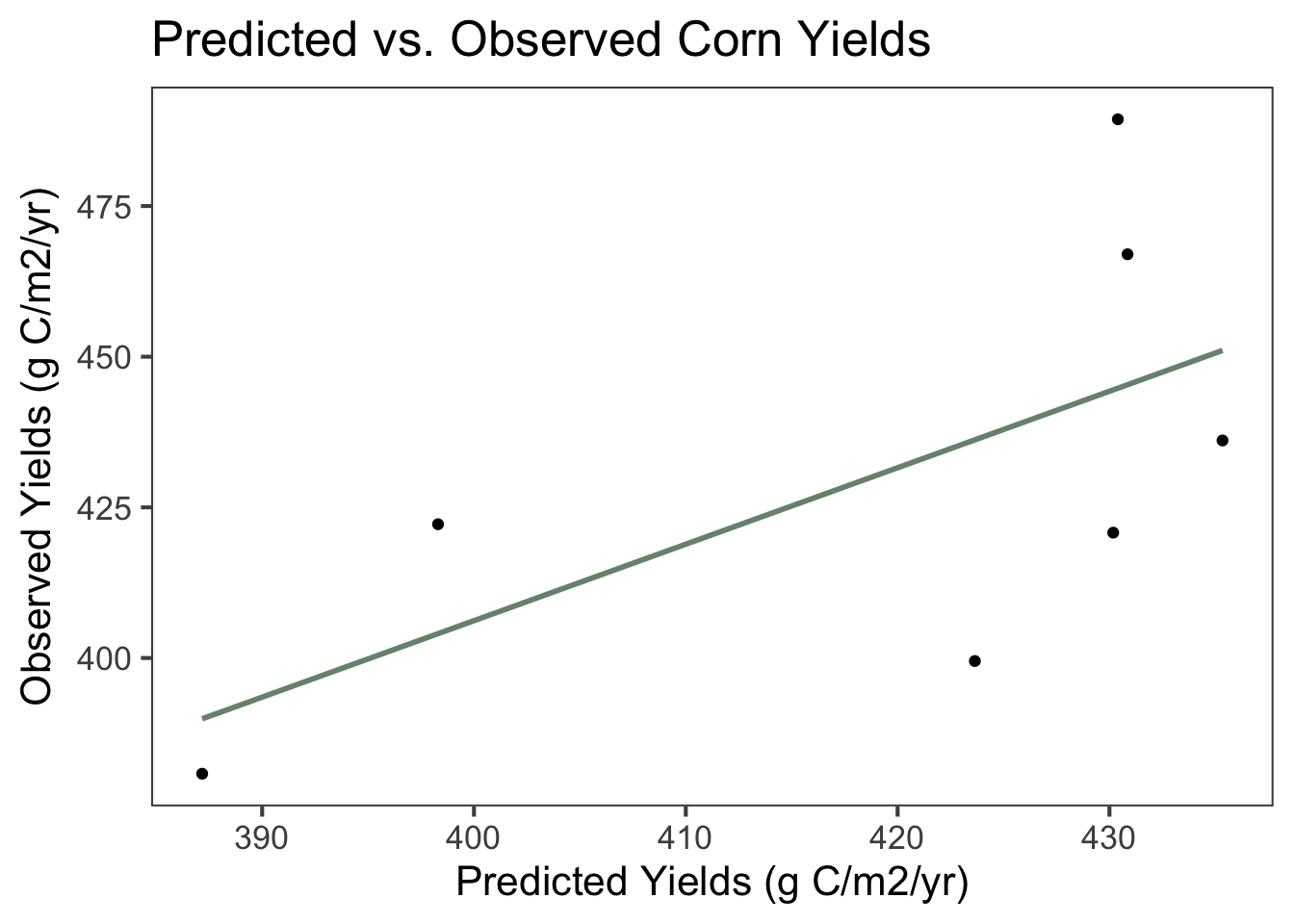

Figure 9.2: Scatterplot and linear regression line of predicted and observed corn yields in grams of carbon (C) per m2 per year between 1999 and 2013. The equation of the line is 0.320x + 282, demonstrating that observed yields were higher than predicted yields on average. The multiple R2 value is 0.406 and the adjusted R2 value is 0.287, indicating that the linear relationship is weak. The p-value is 0.124, a little higher than what is generally considered to be significant.

9.4 Mean, standard deviation, and standard error for predicted and observed outputs

#Summary stats for predicted outputs - mean, sd, se
centwheat %>% # summary stats for CM wheat outputs
  summarise(n = n(),
            mean = mean(cgrain_cent), # mean
            sd = sd(cgrain_cent), # standard deviation
            SE = sd/sqrt(n)) # standard error

##   n     mean       sd       SE
## 1 8 355.2258 29.86568 10.55911

centcorn %>% # summary stats for CM corn outputs
  summarise(n = n(),
            mean = mean(cgrain_cent), # mean
            sd = sd(cgrain_cent), # standard deviation
            SE = sd/sqrt(n)) # standard error

##   n     mean       sd       SE
## 1 7 419.4124 18.81556 7.111612

#Summary stats for observed outputs - mean, sd, se
obswheat %>% # summary stats for observed wheat outputs
  summarise(n = n(),
            mean = mean(cgrain_obs), # mean
            sd = sd(cgrain_obs), # standard deviation
            SE = sd/sqrt(n)) # standard error

##   n  mean       sd       SE
## 1 8 359.7 30.74364 10.86952

obscorn %>% # summary stats for observed corn outputs
  summarise(n = n(),
            mean = mean(cgrain_obs), # mean
            sd = sd(cgrain_obs), # standard deviation
            SE = sd/sqrt(n)) # standard error

##   n     mean       sd       SE
## 1 7 430.8286 37.47473 14.16412

9.5 Model evaluation via Mean Absolute Error (MAE) and Root Mean Squared Error (RMSE)

#Model evaluation stats
mae(centgrain13[,3], obsgrain[,3]) # mean absolute error for predicted vs. observed yields

## [1] 32.46613

rmse(centgrain13[,3], obsgrain[,3]) # root mean squared error for predicted vs. observed yields

## [1] 40.71014

From the MAE, we see that the average amount that predicted values deviated from observed values in either the positive or negative direction was 32.47. If the RMSE was close or equal to the standard deviations of observed data, then the model would be considered a good fit. In this case, the RMSE is much higher than the standard deviations. From this and the low significance of the linear regression models, we can see that the Century Model was not a very good fit with the observed data.