Chapter 5 Extracting and Visualizing Meteorological Data

“What do you call dangerous precipitation? A rain of terror.”

For this assignment, we used custom functions to read in and look at average meteorological data scraped from a public data archive.

Data is from Snowstudies.org. Assignment by Dr. Matthew Ross and Dr. Nathan Mueller of Colorado State University.

5.1 Extract the meteorological data URLs.

# Read HTML page 
snowarchive <- read_html("https://snowstudies.org/archived-data/")

# Read link with specific pattern
links <- snowarchive %>%
  html_nodes('a') %>% #look for links
  .[grepl('forcing',.)] %>% #filter to only links with "forcing" term
  html_attr('href') #tell it these are urls

links # view

## [1] "https://snowstudies.org/wp-content/uploads/2022/02/SBB_SASP_Forcing_Data.txt"
## [2] "https://snowstudies.org/wp-content/uploads/2022/02/SBB_SBSP_Forcing_Data.txt"

5.2 Download the meteorological data from the URL

# Grab only the name of the file by splitting out on forward slashes
splits <- str_split_fixed(links,'/',8)

#Keep only the 8th column
files <- splits[,8] 

files

## [1] "SBB_SASP_Forcing_Data.txt" "SBB_SBSP_Forcing_Data.txt"

# Generate a file list for where the data goes
file_names <- paste0('Data_sci_bookdown/data/snow/', files)

# For loop that downloads each - i for every instance, length function tells how many instances
for(i in 1:length(file_names)){
  download.file(links[i],destfile=file_names[i])
}

# Download via map function
#map2(links, file_names, download.file)

# Map version of the for loop (downloading files)
downloaded <- file.exists(file_names) 
evaluate <- !all(downloaded) # sees if files are downloaded (T/F)
if(evaluate == T){
  map2(links[1:2],file_names[1:2],download.file)
}else{print('data downloaded')}

## [1] "data downloaded"

5.3 Write a custom function to read in the data and append a site column to the data

# Traditional read in

SASP <- read.csv("Data_sci_bookdown/data/snow/SBB_SASP_Forcing_Data.csv") %>%
  select(1,2,3,7,10)
  
colnames(SASP) <- c("year","month","day","precip","temp")

SBSP <- read.csv("Data_sci_bookdown/data/snow/SBB_SBSP_Forcing_Data.csv") %>%
  select(1,2,3,7,10)
  
colnames(SBSP) <- c("year","month","day","precip","temp")

# Combine csvs
alldata <- rbind(SASP,SBSP)

# Read in via new function

# Grab headers from metadata pdf
library(pdftools)

## Using poppler version 20.12.1

headers <- pdf_text('https://snowstudies.org/wp-content/uploads/2022/02/Serially-Complete-Metadata-text08.pdf') %>%
  readr::read_lines(.) %>%
  trimws(.) %>%
  str_split_fixed(.,'\\.',2) %>%
  .[,2] %>%
  .[1:26] %>%
  str_trim(side = "left")

5.4 Use the map function to read in both meteorological files

# Pull site name out of the file name and read in the .txt files
read_data <- function(file){
  name = str_split_fixed(file,'_',2)[,2] %>% 
    gsub('_Forcing_Data.txt','',.) 
  df <- read_fwf(file) %>% 
    select(year=1, month=2, day=3, hour=4, precip=7, air_temp=10) %>% #choose and name columns
    mutate(site = name) #add column 
}

alldata2 <- map_dfr(file_names,read_data) 

## Rows: 69168 Columns: 19
## ── Column specification ────────────────────────────────────────────────────────
## 
## chr  (2): X12, X14
## dbl (17): X1, X2, X3, X4, X5, X6, X7, X8, X9, X10, X11, X13, X15, X16, X17, ...
## 
## ℹ Use `spec()` to retrieve the full column specification for this data.
## ℹ Specify the column types or set `show_col_types = FALSE` to quiet this message.
## Rows: 69168 Columns: 19
## ── Column specification ────────────────────────────────────────────────────────
## 
## chr  (2): X12, X14
## dbl (17): X1, X2, X3, X4, X5, X6, X7, X8, X9, X10, X11, X13, X15, X16, X17, ...
## 
## ℹ Use `spec()` to retrieve the full column specification for this data.
## ℹ Specify the column types or set `show_col_types = FALSE` to quiet this message.

summary(alldata2)

##       year          month             day             hour      
##  Min.   :2003   Min.   : 1.000   Min.   : 1.00   Min.   : 0.00  
##  1st Qu.:2005   1st Qu.: 3.000   1st Qu.: 8.00   1st Qu.: 5.75  
##  Median :2007   Median : 6.000   Median :16.00   Median :11.50  
##  Mean   :2007   Mean   : 6.472   Mean   :15.76   Mean   :11.50  
##  3rd Qu.:2009   3rd Qu.: 9.000   3rd Qu.:23.00   3rd Qu.:17.25  
##  Max.   :2011   Max.   :12.000   Max.   :31.00   Max.   :23.00  
##      precip             air_temp         site          
##  Min.   :0.000e+00   Min.   :242.1   Length:138336     
##  1st Qu.:0.000e+00   1st Qu.:265.8   Class :character  
##  Median :0.000e+00   Median :272.6   Mode  :character  
##  Mean   :3.838e-05   Mean   :272.6                     
##  3rd Qu.:0.000e+00   3rd Qu.:279.7                     
##  Max.   :6.111e-03   Max.   :295.8

5.5 Make a line plot of mean temp by year by site

temp_yearly <- alldata2 %>% 
group_by(year, site) %>%
summarise(mean_temp = mean(`air_temp`, na.rm=T))

## `summarise()` has grouped output by 'year'. You can override using the `.groups`
## argument.

ggplot(temp_yearly,aes(x=year, y=mean_temp, color=site)) + 
  geom_point() + geom_line() +
  xlab("Year") + ylab("Mean Temperature (Degrees Kelvin)") +
  ggthemes::theme_few() + 
  scale_color_brewer(palette = "Set2") + 
  scale_x_continuous(breaks = pretty(c(2003,2012), n = 6)) +
  theme(legend.position="bottom")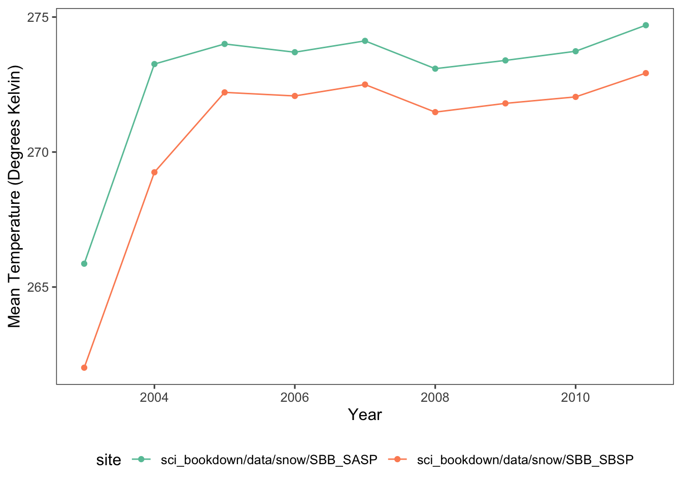

Figure 5.1: Mean temperature of the SASP (teal) and SBSP (orange) sites from 2003 to 2012, in degrees Kelvin.

5.6 Write a function that makes line plots of monthly average temperature at each site for a given year. Use a for loop to make these plots for 2005 to 2010.

temp_monthly <- alldata2 %>%
    group_by(year, month, site) %>%
    summarize(mean_temp = mean(`air_temp`, na.rm=T))

## `summarise()` has grouped output by 'year', 'month'. You can override using the
## `.groups` argument.

par(mfrow=c(5,1))

plot_monthly <- function(year.no) {
  plot <- temp_monthly %>%
    filter(year == year.no) %>%
    ggplot(aes(x=month, y=mean_temp, color=site)) + 
      geom_line() +
      xlab("Month") + ylab("Mean Temperature (Degrees Kelvin)") +
      ggthemes::theme_few() + 
      scale_color_brewer(palette = "Set2") + 
      scale_x_discrete(limits = c(1,2,3,4,5,6,7,8,9,10,11,12)) +
      scale_y_continuous(breaks = pretty(c(255,290), n = 4)) +
      theme(legend.position="bottom")
  print(plot)
  }

for(i in 2005:2010){
  plot_monthly(i)
}

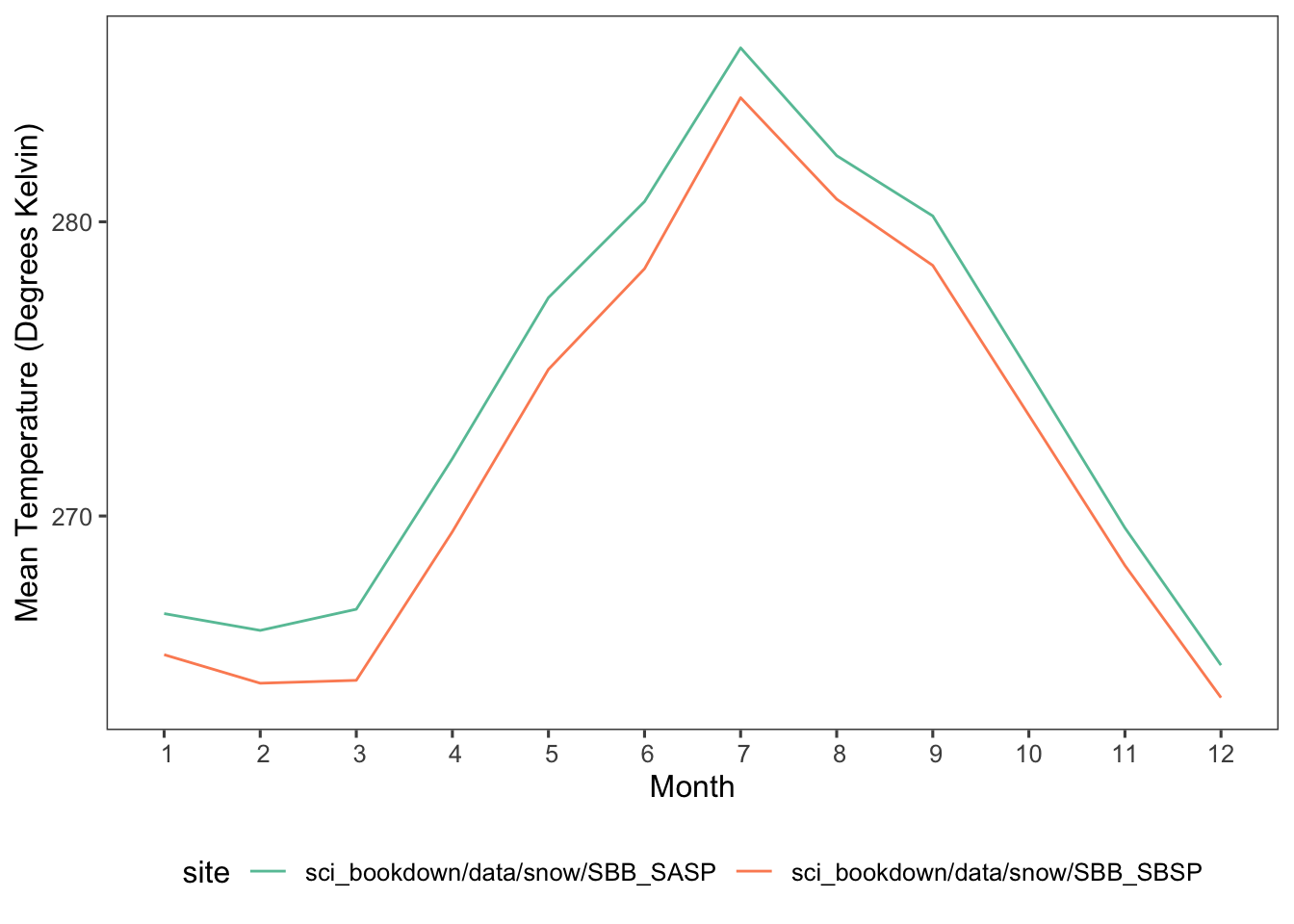
Figure 5.2: Mean monthly temperatures in degrees Kelvin for SASP (teal) and SBSP (orange) sites in 2005, 2006, 2007, 2008, 2009, and 2010.

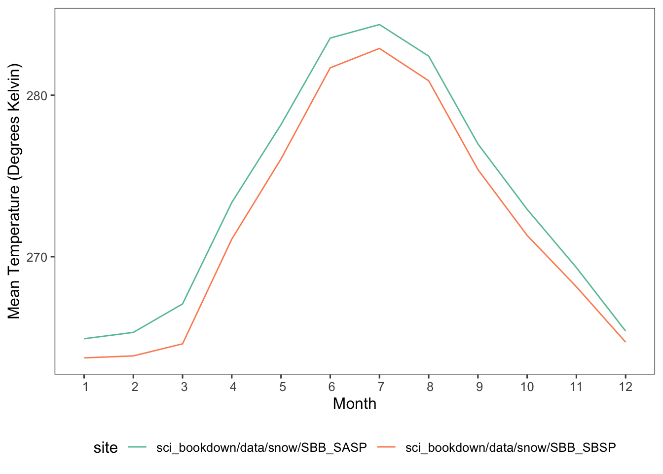
Figure 5.3: Mean monthly temperatures in degrees Kelvin for SASP (teal) and SBSP (orange) sites in 2005, 2006, 2007, 2008, 2009, and 2010.

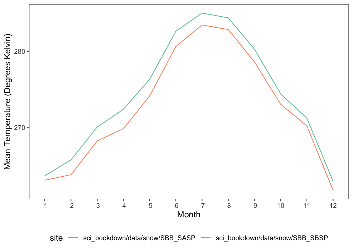
Figure 5.4: Mean monthly temperatures in degrees Kelvin for SASP (teal) and SBSP (orange) sites in 2005, 2006, 2007, 2008, 2009, and 2010.

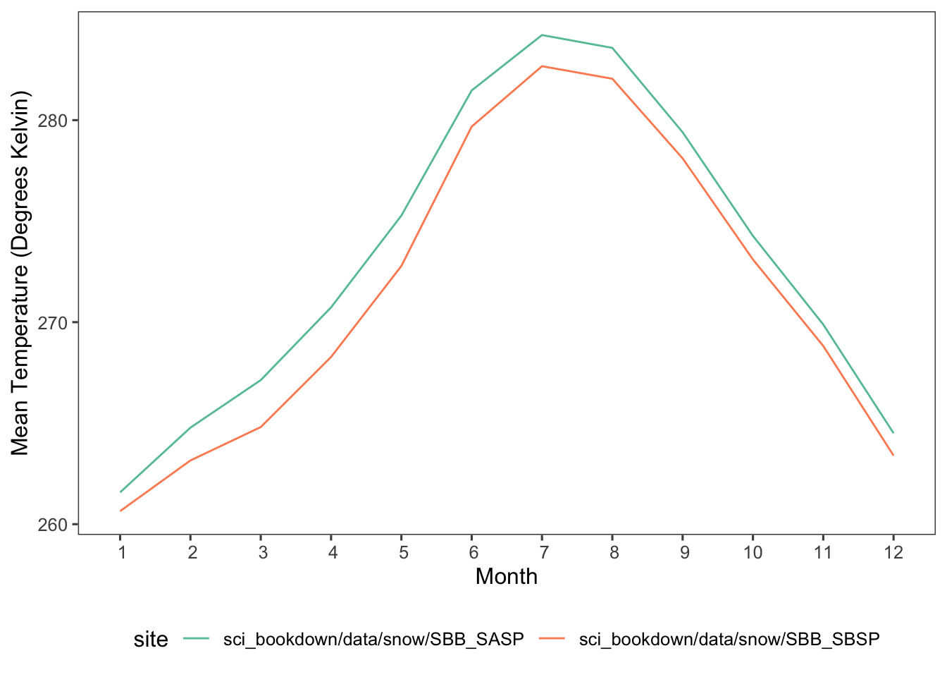
Figure 5.5: Mean monthly temperatures in degrees Kelvin for SASP (teal) and SBSP (orange) sites in 2005, 2006, 2007, 2008, 2009, and 2010.

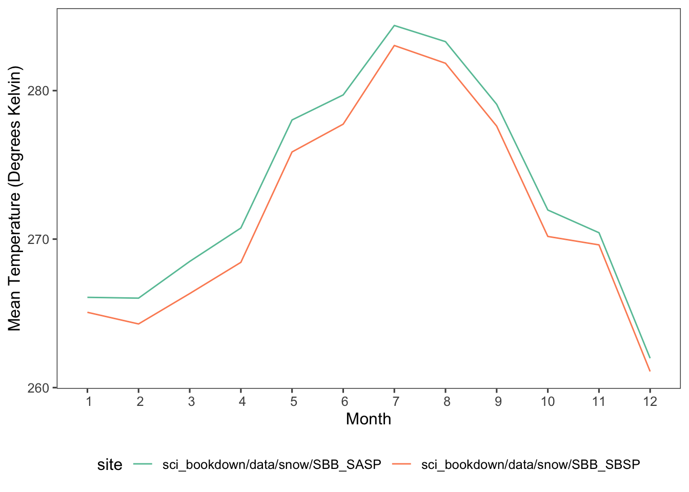
Figure 5.6: Mean monthly temperatures in degrees Kelvin for SASP (teal) and SBSP (orange) sites in 2005, 2006, 2007, 2008, 2009, and 2010.

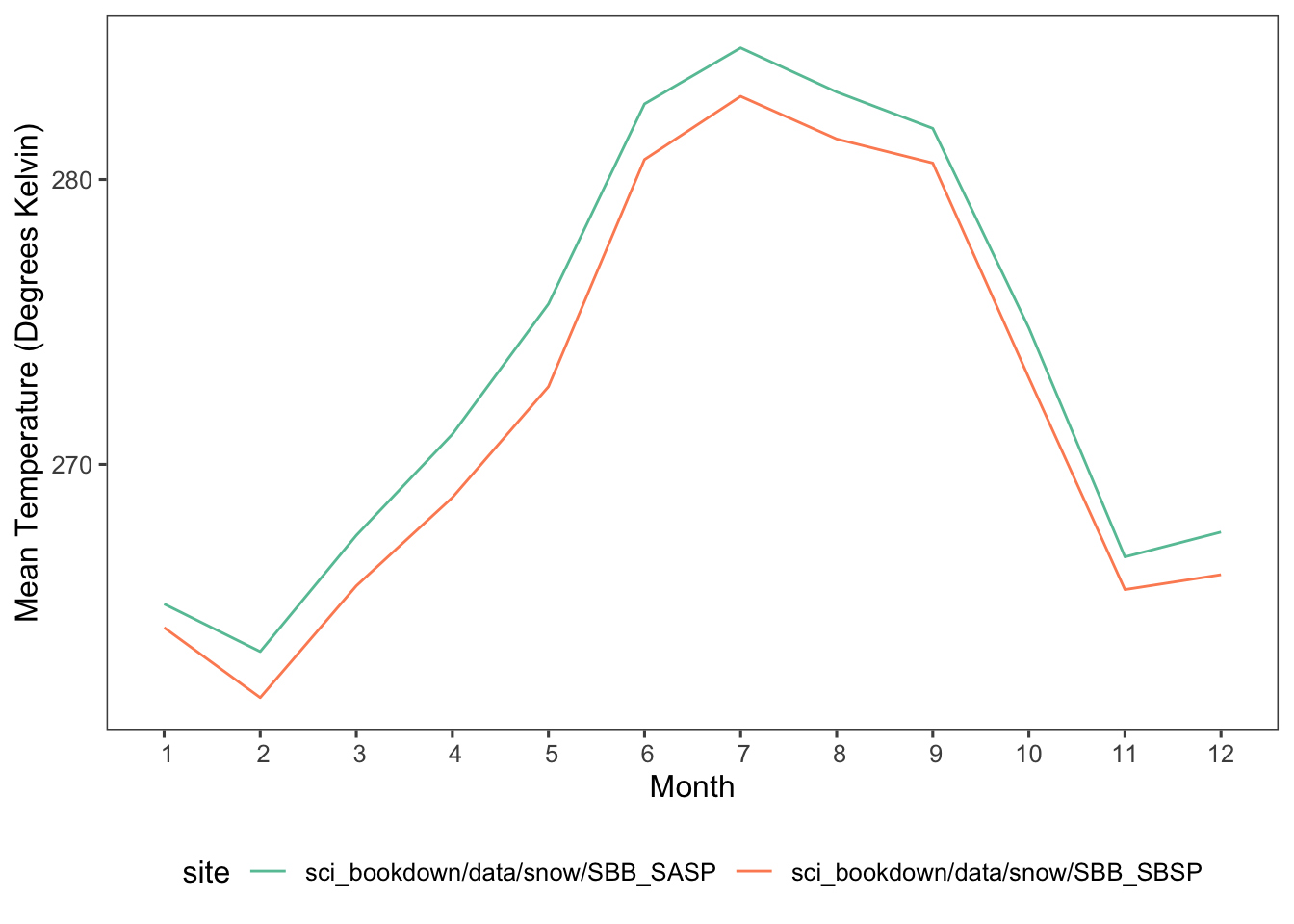
Figure 5.7: Mean monthly temperatures in degrees Kelvin for SASP (teal) and SBSP (orange) sites in 2005, 2006, 2007, 2008, 2009, and 2010.

5.7 Make a plot of average daily precipitation by day of year (averaged across all available years)

precip_daily <- alldata2 %>%
  mutate(date = make_date(year, month, day),
                day_no = yday(date)) %>%
  group_by(day_no) %>%
  summarize(mean_precip = mean(`precip`*86400, na.rm=T))

ggplot(precip_daily, aes(x=day_no, y=mean_precip)) + 
      geom_line() +
      xlab("Day of Year") + ylab("Mean Precipitation (mm/day)") +
      ggthemes::theme_few() + 
      scale_color_brewer(palette = "Set2") + 
      scale_y_continuous(breaks = pretty(c(0,14), n = 7)) +
      scale_x_continuous(breaks = pretty(c(1,365), n = 8))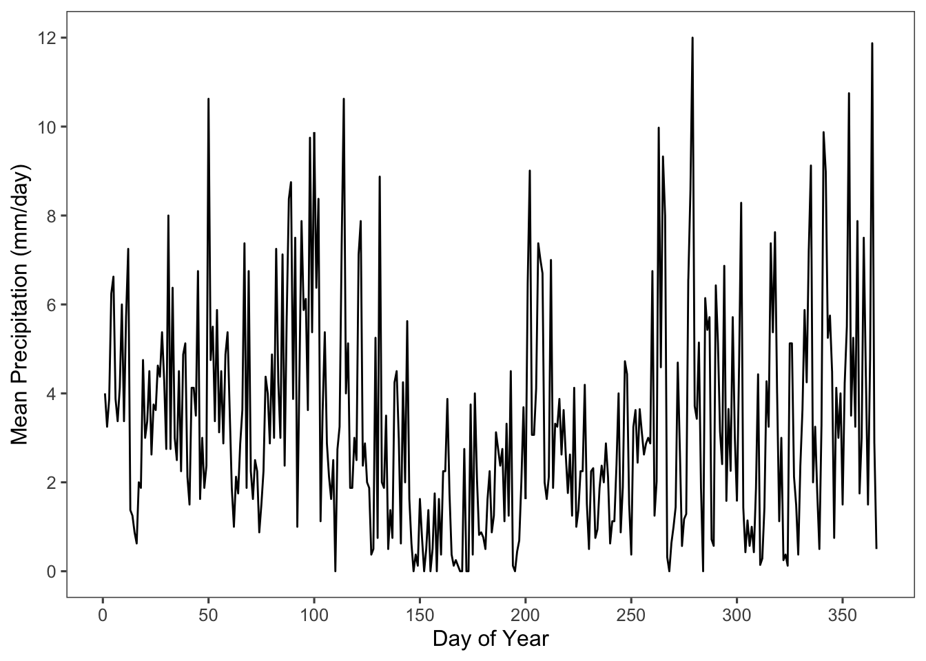

Figure 5.8: Mean daily precipitation by day of year, averaged from 2003 to 2012.