Chapter 4 Fire Effects on Fish Populations
“Where do fish keep their money? In the riverbank.”
Wildfires don’t only impact vegetation, but a wide variety of abiotic and biotic elements of the ecosystem. In this assignment, I looked at how fish in the Cache La Poudre Watershed were impacted by the High Park Fire in 2012.
Data and assignment provided by Dr. Michael Lefsky of Colorado State University.
4.1 Pre versus post fire fish length and mass
#summarize fishdata_R by time (another way to do this without subsets)
summary(fishdata_4R[fishdata_4R$time=="pre-fire",])
## time capture_id length_cm mass_g
## Length:100 Min. : 1.00 Min. : 5.00 Min. : 66
## Class :character 1st Qu.: 25.75 1st Qu.:15.00 1st Qu.:132
## Mode :character Median : 50.50 Median :18.00 Median :151
## Mean : 50.50 Mean :19.16 Mean :154
## 3rd Qu.: 75.25 3rd Qu.:23.00 3rd Qu.:182
## Max. :100.00 Max. :32.00 Max. :252summary(fishdata_4R[fishdata_4R$time=="post-fire",])## time capture_id length_cm mass_g
## Length:97 Min. : 1 Min. : 5.00 Min. : 45.0
## Class :character 1st Qu.:25 1st Qu.:15.00 1st Qu.: 89.0
## Mode :character Median :49 Median :20.00 Median :113.0
## Mean :49 Mean :19.76 Mean :107.9
## 3rd Qu.:73 3rd Qu.:25.00 3rd Qu.:126.0
## Max. :97 Max. :38.00 Max. :157.0# create function to run statistics
lab_stats <- function(x) c(sd(x),sd(x)^2,sd(x)/sqrt(length(x))) #calculate standard deviation, variance, standard error. Return as vector
#Pre-fire statistics
lab_stats(fishdata_4R[fishdata_4R$time=="pre-fire",]$length_cm) #fish length## [1] 6.2145479 38.6206061 0.6214548lab_stats(fishdata_4R[fishdata_4R$time=="pre-fire",]$mass_g) #fish mass## [1] 36.277409 1316.050404 3.627741#Post-fire statistics
lab_stats(fishdata_4R[fishdata_4R$time=="post-fire",]$length_cm) #fish length## [1] 7.0574624 49.8077749 0.7165767lab_stats(fishdata_4R[fishdata_4R$time=="post-fire",]$mass_g) #fish mass## [1] 26.894853 723.333119 2.730759# 1-way ANOVA on pre- vs. post-fire mass and length
summary(aov(fishdata_4R$length_cm~fishdata_4R$time)) #ANOVA for fish length pre vs. post fire## Df Sum Sq Mean Sq F value Pr(>F)
## fishdata_4R$time 1 18 17.90 0.406 0.525
## Residuals 195 8605 44.13summary(aov(fishdata_4R$mass_g~fishdata_4R$time)) #ANOVA for fish mass pre vs. post fire## Df Sum Sq Mean Sq F value Pr(>F)
## fishdata_4R$time 1 104798 104798 102.3 <2e-16 ***
## Residuals 195 199729 1024
## ---
## Signif. codes: 0 '***' 0.001 '**' 0.01 '*' 0.05 '.' 0.1 ' ' 1# Make a 2 x 2 matrix of histograms for pre- and post-fire mass and length
par(mfrow=c(2,2)) #tell R how I want figures arranged
#Pre-fire histograms
hist(fishdata_4R[fishdata_4R$time == "pre-fire",]$length_cm,main="Pre-fire length (cm)",xlab="Length (cm)") #fish length
hist(fishdata_4R[fishdata_4R$time == "pre-fire",]$mass_g,main="Pre-fire mass (g)",xlab="Mass (g)") #fish mass
#Post-fire histograms
hist(fishdata_4R[fishdata_4R$time == "post-fire",]$length_cm,main="Post-fire length (cm)",xlab="Length (cm)") #fish length
hist(fishdata_4R[fishdata_4R$time == "post-fire",]$mass_g,main="Post-fire mass (g)",xlab="Mass (g)") #fish mass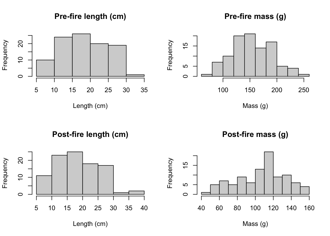
Figure 4.1: Histograms showing frequency of various lengths in centimeters and masses in grams of fish in in Cache La Poudre Watershed in 2012 before the High Park Fire (Pre-fire) and in 2013 after the High Park Fire (Post-fire).
# Make a 2 x 2 matrix of histograms for pre- and post-fire mass and length
par(mfrow=c(2,2)) #tell R how I want figures arranged

# Make two boxplots side by side
par(mfrow=c(1,2)) #tell R I want two plots
boxplot(fishdata_4R$length_cm~fishdata_4R$time, main="Length (cm)",ylab = "Frequency",xlab="Time") #length fre and post fire
boxplot(fishdata_4R$mass_g~fishdata_4R$time, main="Mass (g)",ylab = "Frequency",xlab="Time") #length fre and post fire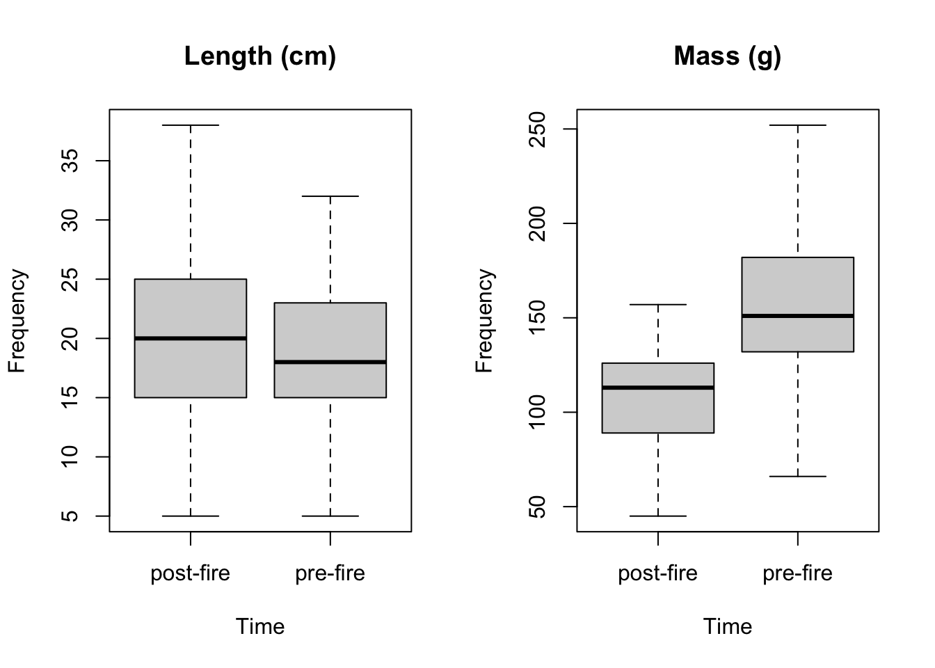
Figure 4.2: Boxplots for fish length in centimeters and mass in grams pre and post fire.
# Reset setting for plots
par(mfrow=c(1,1)) #return to single plot
4.2 Linear regression of fish mass vs. length for before and after the fire
# Pre-fire
# Scatterplot of length and mass where length is the independent variable and mass is the response variable
plot(mass_g ~ length_cm, data=fishdata_4R[fishdata_4R$time=="pre-fire",], xlab="Length (cm)", ylab="Mass (g)")
title("Pre-fire Fish Mass vs. Length")

# Linear regression on mass vs.length
lm_pre <- lm(mass_g ~ length_cm,data=fishdata_4R[fishdata_4R$time=="pre-fire",])
abline(lm_pre)  #Adds the trendline to the regression scatterplot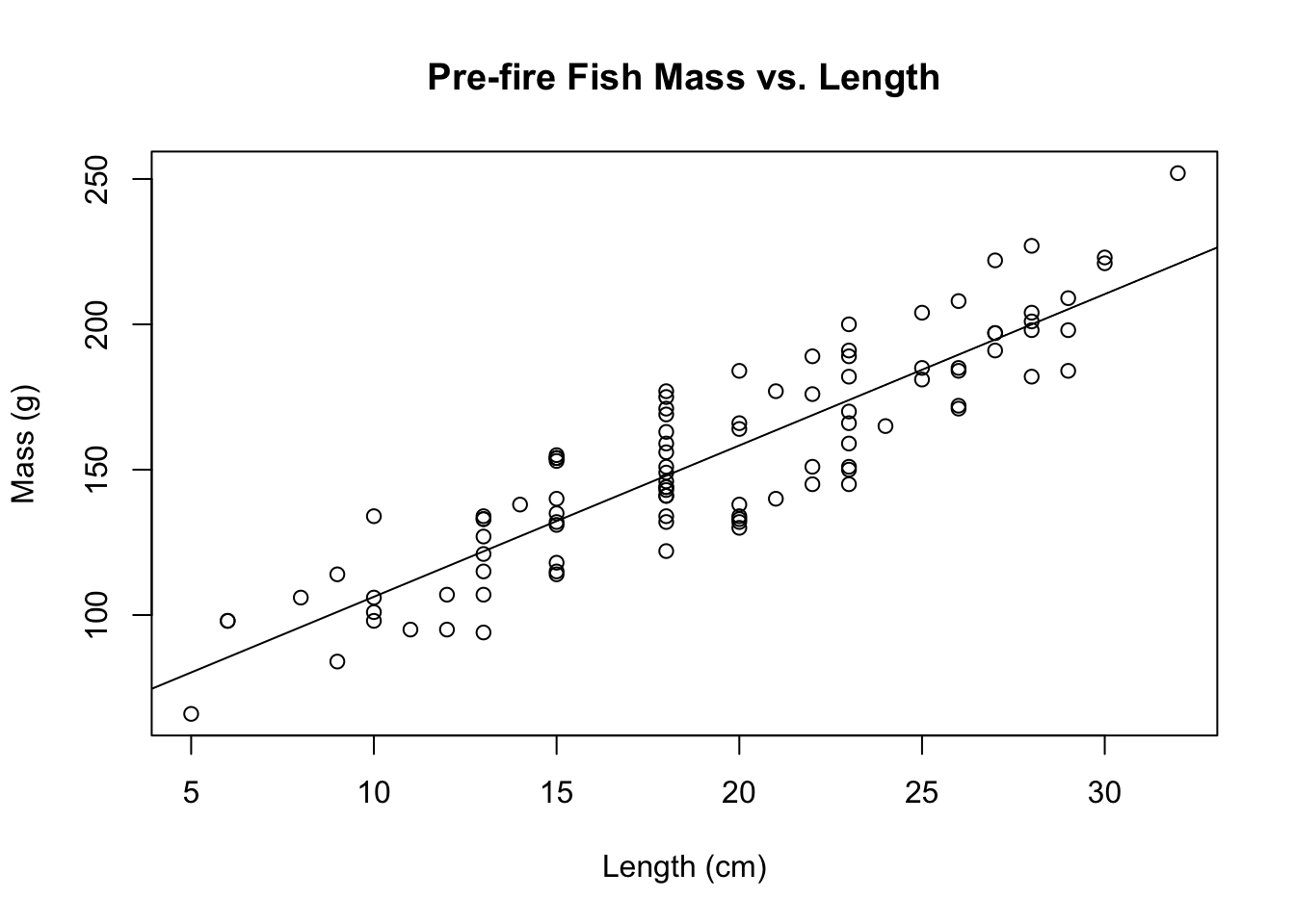
Figure 4.3: Scatterplot and linear regression line of fish length in centimeters versus fish mass in grams in Cache La Poudre in 2012 before the High Park Fire.
summary(aov(lm_pre)) #shows the results of the pre-fire linear regression ANOVA## Df Sum Sq Mean Sq F value Pr(>F)
## length_cm 1 103690 103690 382 <2e-16 ***
## Residuals 98 26599 271
## ---
## Signif. codes: 0 '***' 0.001 '**' 0.01 '*' 0.05 '.' 0.1 ' ' 1summary(lm_pre) #shows equation of the line, multiple R-squared value##
## Call:
## lm(formula = mass_g ~ length_cm, data = fishdata_4R[fishdata_4R$time ==
## "pre-fire", ])
##
## Residuals:
## Min 1Q Median 3Q Max
## -28.987 -14.472 -0.307 12.543 31.144
##
## Coefficients:
## Estimate Std. Error t value Pr(>|t|)
## (Intercept) 54.2113 5.3641 10.11 <2e-16 ***
## length_cm 5.2077 0.2664 19.55 <2e-16 ***
## ---
## Signif. codes: 0 '***' 0.001 '**' 0.01 '*' 0.05 '.' 0.1 ' ' 1
##
## Residual standard error: 16.47 on 98 degrees of freedom
## Multiple R-squared: 0.7958, Adjusted R-squared: 0.7938
## F-statistic: 382 on 1 and 98 DF, p-value: < 2.2e-16# Post-fire
# Scatterplot of length and mass where length is the independent variable and mass is the response variable
plot(mass_g ~ length_cm, data=fishdata_4R[fishdata_4R$time=="post-fire",], xlab="Length (cm)", ylab="Mass (g)")
title("Post-fire Fish Mass vs. Length")
# Linear regression on mass vs.length
lm_post <- lm(mass_g ~ length_cm,data=fishdata_4R[fishdata_4R$time=="post-fire",])
abline(lm_post) #Adds the trendline to the regression scatterplot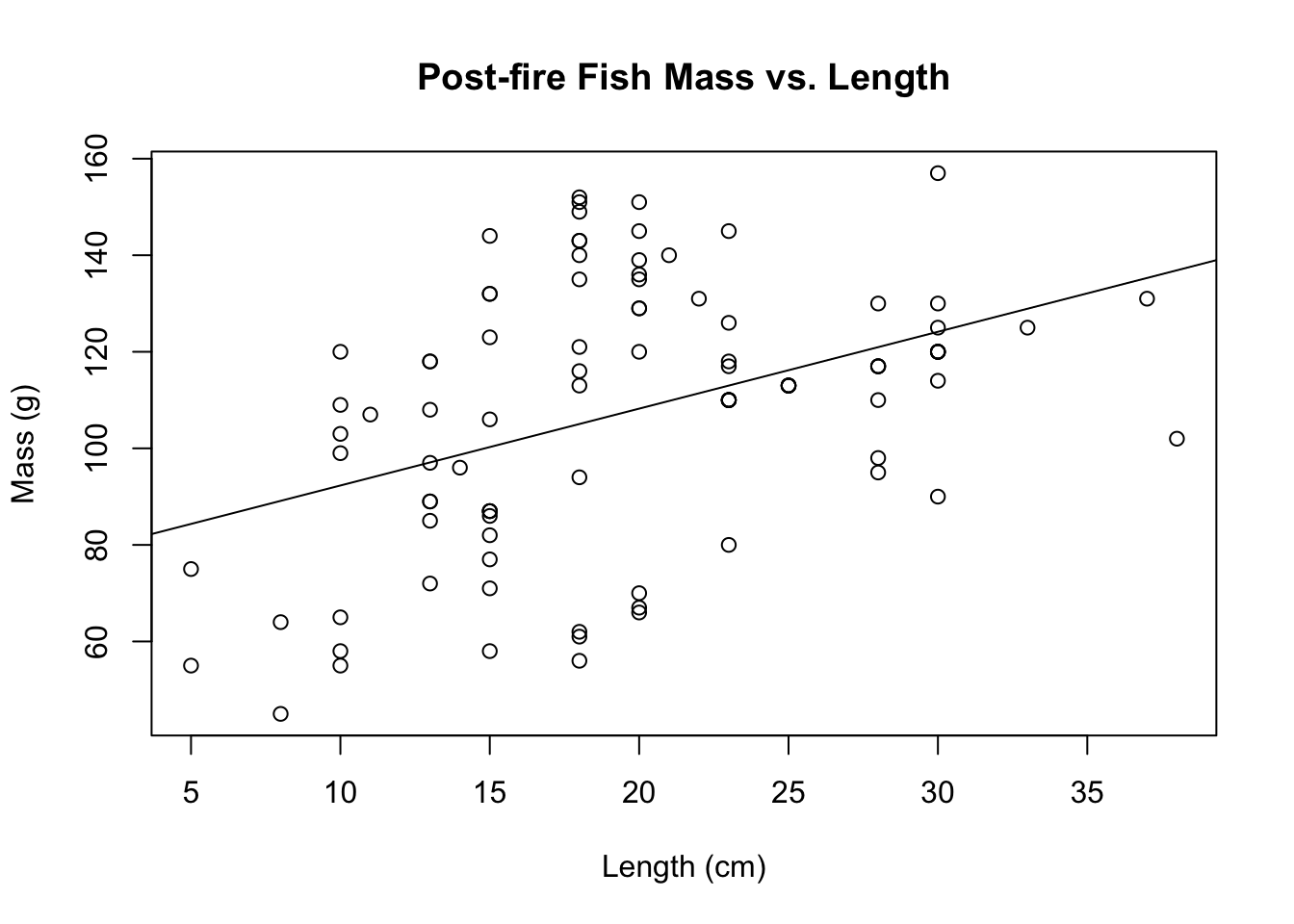
Figure 4.4: Scatterplot and linear regression line of fish length in centimeters versus fish mass in grams in Cache La Poudre in 2013 after the High Park Fire.
summary(aov(lm_post)) #shows the results of the pre-fire linear regression ANOVA## Df Sum Sq Mean Sq F value Pr(>F)
## length_cm 1 12126 12126 20.1 2.05e-05 ***
## Residuals 95 57313 603
## ---
## Signif. codes: 0 '***' 0.001 '**' 0.01 '*' 0.05 '.' 0.1 ' ' 1summary(lm_post) #shows equation of the line, multiple R-squared value##
## Call:
## lm(formula = mass_g ~ length_cm, data = fishdata_4R[fishdata_4R$time ==
## "post-fire", ])
##
## Residuals:
## Min 1Q Median 3Q Max
## -49.048 -13.271 -3.011 19.582 46.952
##
## Coefficients:
## Estimate Std. Error t value Pr(>|t|)
## (Intercept) 76.3830 7.4498 10.253 < 2e-16 ***
## length_cm 1.5925 0.3552 4.483 2.05e-05 ***
## ---
## Signif. codes: 0 '***' 0.001 '**' 0.01 '*' 0.05 '.' 0.1 ' ' 1
##
## Residual standard error: 24.56 on 95 degrees of freedom
## Multiple R-squared: 0.1746, Adjusted R-squared: 0.1659
## F-statistic: 20.1 on 1 and 95 DF, p-value: 2.054e-05#Pre- and Post-Fire on same graph
# First plot the pre-fire linear regression
# ylim sets the range of the y-axis; pch="+" makes points appear as plus signs; col="blue" makes plus signs blue
plot(mass_g ~length_cm,data=fishdata_4R[fishdata_4R$time == "pre-fire",],xlab="Length (cm)",ylab="Mass (g)",ylim=c(0,260), pch="+", col="blue")
title("Pre-Fire (+) and Post-Fire (o) Mass vs. Length")
# Run linear regression of pre-fire mass and length to obtain the trend line.
lm_pre=lm(mass_g ~ length_cm,data=fishdata_4R[fishdata_4R$time == "pre-fire",])
abline(lm_pre,col="blue") #adds a trendline to the plot and makes the line blue
# Overlay the post-fire linear regression onto the plot of the pre-fire linear regression
# Plots post-fire data as o's and colors them red
points(mass_g ~length_cm,data=fishdata_4R[fishdata_4R$time == "post-fire",],xlab="Length (cm)",ylab="Mass (g)",ylim=c(0,260),col="red")
# Run linear regression of post-fire mass and length to obtain the trend line.
lm_post=lm(mass_g ~ length_cm,data=fishdata_4R[fishdata_4R$time == "post-fire",])
abline(lm_post,col="red") #adds a trendline to the post-fire linear regression and makes the line red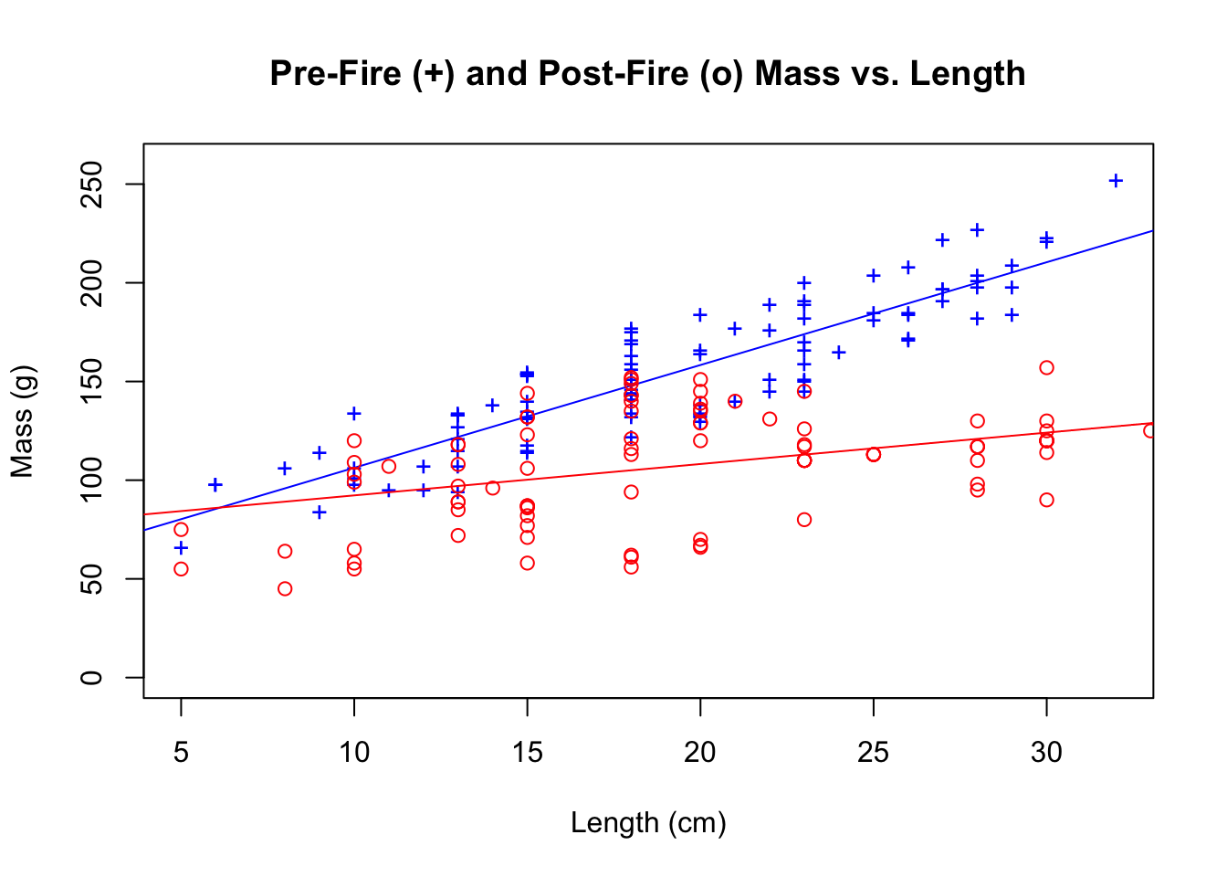
Figure 4.5: Scatterplot and linear regression line of fish length in centimeters versus fish mass in grams in Cache La Poudre in 2012 before the High Park Fire (blue, +) and in 2013 after the High Park Fire (red, o).